
From this article, you will learn how to sum alternative rows/ columns in Excel with help of SUMIF Function.
Excel has various functions, including functions to calculate the inverse cosine of a given value, to multiply matrices, to estimate the internal rate of return. But, most of us use just about 5-6 formulas to do our jobs. And IF formulas are a majority of these, so very useful to learn a few interesting things you can do with just the excel IF functions.
Sometimes when you are working on data and required to sum alternate Rows Or Columns. Now we can various way to calculate alternate rows or columns data.
Syntax : = SUMIF (range, criteria, [sum_Range])
Table of Contents
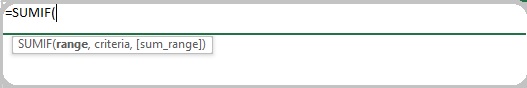
Range: The Range of cells that you want to calculate by criteria. Cells in each range must be numbers or names, arrays, or references that contain numbers. Blank and text values are ignored. The selected range may contain dates in standard Excel format.
Criteria: The Criteria is in the form of number, name, text, function that defines which cells will be added.
Wildcard characters can be included – a question mark (?) to match any single character, an asterisk (*) to match any sequence of characters. If you want to find an actual question mark or asterisk, type a tilde (~) preceding the character.
For example, criteria can be used as 32, “40”, B5, “2?”, “Team1*”, “*~?”, or TODAY().
Sum_Range: The Actual cells to be added, Sum range should be the same as the range.
How to Sum alternative Rows or Column:
Let’s Understand with Below Given Data:

In the above-given data, there is one revenue detail. Now we have to calculate alternate rows revenue. So what we have to do?
First of all you have mention 0 & 1 in the next column for every cell. Just enter 1 and 0 in the first 2 rows and then drag till the end or paste simply.
Now Use this column to test our condition by using function. = SUMIF (range, criteria, [sum_Range]).
In our Case formula to be =SUMIF(D3:D14,1,C3:C14)
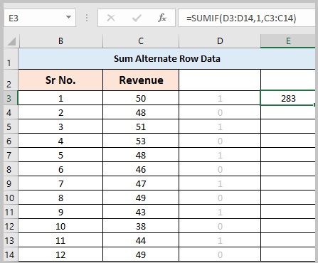
Result of a Function is 283.
Now understand how it is calculated by SUMIF Function. We select D3:D14 as the Range to evaluate the criteria. We have taken 1 as our Criteria for SUM_RANGE of C3:C14. So once we execute the function, it searches 1 number in cells between D3:D14 and sums those row’s data of cells between C3:C14.