How to select every alternate row in excel
Table of Contents
Many times we have required to select every alternate row for highlight or delete it.
even sometimes we download data from where row after every row blank which we need to delete for further work.
Another situation where we need to select alternate row and copy data and paste it to other worksheets.
so let’s learn how to select every other row in excel.
If you have small data set or few line items in worksheet then fastest method to select every other row in excel would be select it manually.
to perform this, you have to use keyboard and mouse/touchpad as well.
Below, I have a one small dataset where I want to select every alternate row.
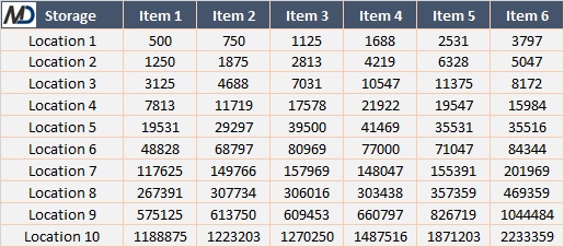
Select Every Alternate/Other row manually
Below are the steps, follow this:
- Press Control key (CTRL) in keyboard and keep holding it.
- Click on Row header of the row that you would like to select ( In our example, it would be row no 4, which is second row of our data set).
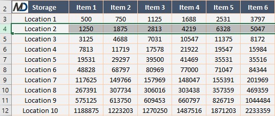
- Continue hold CTRL key and then click the row header of all the rows that you want to select. Do not leave CTRL until all row selected.
- Once all rows selected then leave CTRL key.
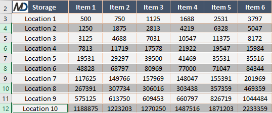
Above given method help you to work when you have a small data set to work.
Select Alternate Row using Helper Column & Filter method
Another method to select every other row in excel is simply we need to add one helper column in data set and then using helper column to filter so that only those rows are available which we have to select.
Let’s understand with an example.
I have below attached data set where I want to select every alternate row.
Here are the steps to follow for execute a helper and filter functionality.
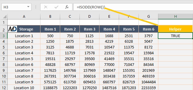
- Enter the Text Helper in Cell H2. It would be our helper column in data set.
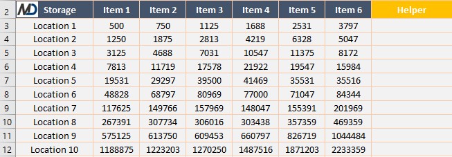
- In Cell H3, enter below given formula.
=ISODD(ROW())
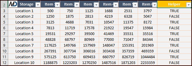
Copy above given formula in all rows of data set.
This formula uses the ISODD function with the ROW function to give TRUE if the row number is odd else FALSE. - Select any row in Helper column and click on Data Tab.
- Click on the Filter Icon in the Sort & Filter group. This will add filter icon in data set. We can use short cut CTRL+ALT+L for filter.
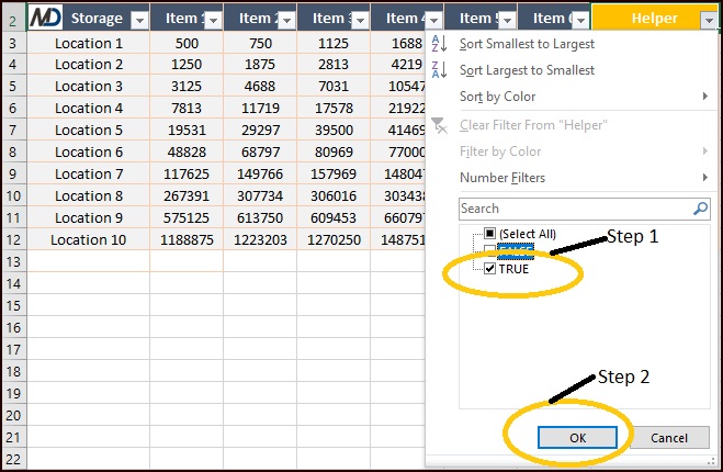
- Click on the filter icon in helper row column header.
- Untick FALSE option and click OK. This will filter your data set. You will see only those rows where the value will be TRUE in helper column.
Same way you can select FALSE as per requirement. - Select the Data set, which is available after filter.
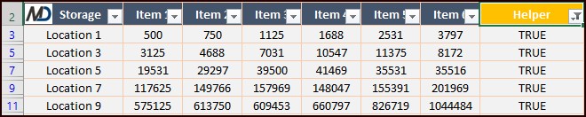
Now you select the cells which are visible in data set that only selected.
So anything you do with data set would not impact to other data which are not visible.